
It’s 2020 and so much has changed, while we aren’t quite yet living like the Jetson’s with our flying cars, alot of progress has been made. Look around you: from driverless cars, using face recognition to unlock your smart phone, and automatic facebook tags. Image classification is in full use. We even use image classification to identify sicknesses such as pneumonia or cancer. How do computers do this? The answer lies in Convolutional Neural Networks or CNNs.
But before we begin, lets talk about the human neuron….
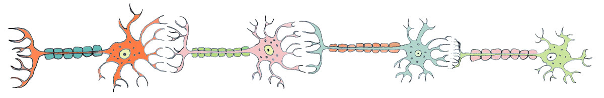
Your crash course to human neurons is this:
Neurons are specialized cells in your body that use electrial impluses to send chemical signals from your brain to the rest of your body. They are the reason you can do pretty much anything. As shown in the image above, multiple neurons link together and these signals jump from one neuron to the next. Neurons have a part of them called receptors. These receptors receive the information, process it, and then send it on to the next neuron. This means that each piece of information is not necessarily moved forward, but only the important messages that will have an impact on the body. (If you are interested look up inhibitors and excitatory neurotransmitters.) So what does this have to do with convolutional neural networks?
A LOT
Convolutional Neural Networks process pretty much the same way as the neurons in our brains. Neural networks are structured in different layers that receive an input that needs to be passed through to each layer. In the case of CNN’s its an image. Each part of the image has a specfic weight, the higher the weight the stronger that signal is and it gets pushed through to the next layer. In the image below, do you see how just with a neuron there is an input into the Convolutional Neural Network? In this case it is an image of a car.

The second layer or “neuron” would be the convolution layer. Seen in the gif below this layer reads the image a section at a time (usually sized 3x3 or 5x5) and moves right until it completes the width of the image. It then moves down a row and completes the same process until the entire image is read.

You may notice in the above car image that there is more than one convolution layer present. These layers operate similarly except that the earlier layer will capture low-level features like color, edges, and gradient orientation. As we move onto the next convolutional layer the details become more complex. There is potential for errors with convolutional layers including image shrinking or the edges becoming less clear. To help fight against this the data scientist can use something called padding. Padding is basically adding a layer of pixels around the edge of an image in order to preserve the true size of the image when convolution is occurring.
Up next we can see the pooling layer. This layer is used to reduce the spatial size of the previous convolutional layer. By downsampling the convolutional layer it aids in decreasing the computational power required to execute the model as well as helping aid against over-fitting the model. The two different types of pooling are Max pooling and Average pooling. As shown above Max pooling returns the maximum value from each portion of the image. In the image, we can see Max pooling returns 100, 184, 12, and 45 which are all the highest number in their respective portion. Average Pooling takes the average of all the values in each portion of the image. If we were to add the green numbers up and divide by four we would get 36. Max pooling is the most popular version of pooling to use because of its higher success rate.
Important parameters to discuss in pooling is pool size and stride. Pool size is the “window size over which to take the maximum (2, 2) will take the max value over a 2 x 2 pooling window. If only one interger is specified the same window length will be used for all dimensions.” (tensorflow.org) Stride specifies “how far the pooling window moves for each pooling step.” (tensorflow.org).

Last, but not least is our fully connected layer. Now that we have ran the convolutional and pooling layers we need to flatten our image into a column vector. This flattened vector is fed into the neural network and backpropagation is applied. The CNN has now looked at high level and low level features in the images and can begin distinguishing between the images or objects. As seen above the CNN uses flattening in order to predict that the image shows a picture of a cat rather than a dog.
Convolutional Neural Networks hold so much potential for the future. From advances in cars, phones, medicine, and banking safety, there are countless items we can look into. Long story short, it might not be too long until we are flying with the Jetsons.
Sources:
https://medium.com/towards-artificial-intelligence/convolutional-neural-networks-for-dummies-afd7166cd9e
https://towardsdatascience.com/a-comprehensive-guide-to-convolutional-neural-networks-the-eli5-way-3bd2b1164a53
https://learn.co/tracks/module-4-data-science-career-2-1/appendix/convolutional-neural-networks/convolutional-neural-networks
https://www.quora.com/What-is-max-pooling-in-convolutional-neural-networks
https://www.tensorflow.org/api_docs/python/tf/keras/layers/MaxPool2D