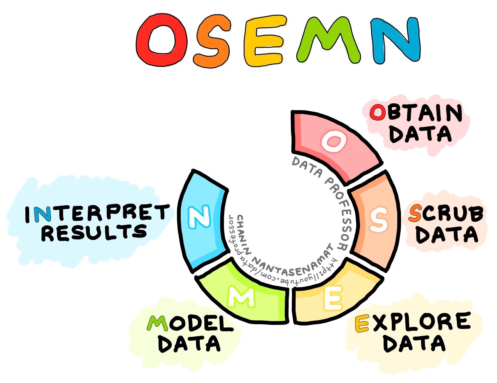
There are many popular processes for a data scientist to go through in order to complete their work, one of the most popular in the field at this time is a strategy classed OSEMN (rhymes with awesome). Today we will cover the five steps of OSEMN and why it is such a useful tool for data scientists.
(Drawn by Chanin Nantasenamat)
O - Obtaining Data
Obtaining data can be performed in a variety of ways. Depending on what company you are working for they may provide the data for you, if not you will most likely need to web scrape, use an API, or be familiar with SQL. Once the data is obtained, it is important to take a look at what you have acquired and become familiar with your dataset. Some helpful strategies to use are:
df.head() - Provides first five rows of data frame.
df.info() - Shows if there are any missing entries within the columns, identifies data type, and provides number of columns.
df.describe() - Gives count, mean, std, min, 25%, 50%, 75%, and max per column.
S - Scrub Data
Scrubbing data is one of the most time consuming aspects of a data scientist’s career. However, it is crucial to get the data into a format that is easier to use. Within most obtained data there will be something missing or wrong with it. Common items to look out for are null values, abnormal numbers, symbols, or data types that must be converted. When identifying nulls it is essential to decide how you are going to handle them. Code that is commonly used for handling null values is listed below:
df.isna().sum() - Allows you to see the quantity of null values in your data frame per column.
df.unique() - Allows you to see the unique items per column.
df.nunique() - Totals the number of unique items for you.
df.fillna() or df.replace() - Are great tools for filling or replacing your nulls with something else.
df.drop() - If you would like to drop an entire row or column for excessive null values.
To switch data type:
df.col = df.col.astype('new_data_type')
Other items to look for while scrubbing the data are categorical variables (sometimes this is done within the exploration step).
cat_cols = df.select_dtypes('object').columns - identifies any categoricals listed as an object. You will have to get familiar with your dataset to see if any categoricals are listed as numerical columns; common examples of these would be zipcode, age group, and education level.
Additional Scrubbing for a Linear Regression Model
Check for multicollinearity:
data = df.iloc[:, 1:20]- Choose columns to check for multicollinearity, then drop whatever the dependent value is.data.corr()abs(data.corr()0 > .75- Take a look at correlation over .75
The next steps use the vif strategy for dealing with multicollinearity. This method is becoming more and more commonly used in the data scientist field.
from statsmodels.stats.outliers_influence import variance_inflation_factorX = data.drop('dependent_col', axis=1)X = sm.add_constant(X)X.shapevif = [variance_inflaction_factor{X.values, i) for i in range(X.shape[1])]vif_results = pd.Series(dict(zip(X.columns, vif)))vif_results- Next we are going to look for any vif with a thershold over 6. The number 6 is a cut off point for multicollinearity.
threshold = 6bad_vif = list(vif_results[vif_results>threshold].index)` if’const’ in bad_vif:- Then drop the bad vif columns from your data frame.
Depending on preference it is very common to run mutliple models in order to see the R2 and multicollinearity changes throughout your work flow. You may have to check multicollinearity multiple times as you manipulate your data. Next we will run through how to normalize your data. Two popular methods are using z-score or the data’s IQR. I will be modeling the IQR method below:
Q1 = data['dependent_col'].quantile(0.25)Q3 = data['dependent_col'].quantile(0.75)IQR = Q3-Q1print(IQR)test = df_ohe[~((df_ohe['price'] < (Q1 - 1.5 * IQR)) |(df_ohe['price'] > (Q3 + 1.5 * IQR)))]print(df_out.shape)- Save a new dataframe with everything but your outliers. ~ sign means the opposite of, so by adding this in we save everything but the outleirs.
Explore
Explore is where the data scientist will perform their EDA (Exploratory Data Analysis), which is another way of saying the data scientist will make visualizations to better understand the data before modeling. Visualizations included in the explore step are often distplots, kernel density estimates, scatterplots, and qqplots (must create OLS Regression before creating QQPlot). The data scientist should be checking for linearity during the Explore step. Often times Scrub and Explore overlap in the OSEMN process. It is in this step that numpy, seaborn, pandas, and scipy come in handy.
Distplot:
sns.distplot(data)
Scatterplot:
sns.scatterplot(data)
Jointplot (Combines Distplot and Scatterplot):
sns.jointplot(data=df, x='col', y='dependent_col', kind='reg')
QQplot:
sm.graphics.qqplot(model.resid, fit=True, line='45')
Kernel Density Estimates:
sns.kdeplot(data)
Model
The goal of modeling in Linear Regression is inference or prediction. Inference is asking “How does X affect Y?” Whereas prediction asks “How can I use X to predict Y?” There will probably be many model’s completed during your work flow, but this is where your final model should be placed. Below I will show you how to create an OLS model.
import statsmodels.formula.api as smf
target = dependent_colfeatures = '+'.join(data.drop(columns = 'dependent_col').columns)formula = target + '~' + featuresmodel = smf.ols(formula, data).fit()
After running your final model you will want to perform Regression Model Validation using sklearn’s train_test_split.
import sklearn.model_selection
import train_test_split
from sklearn.metrics import r2_score
df_train, df_test = train_test_split(data)df_train.shape, df_test.shape- Check shape- Run an OLS model using the train data
y_train_pred = model.predict(df_train)- Do same for y_test_predr2_train = r2_score(df_train['dependent_col'], y_train_pred)- Do same for r2_test
The goal is to have your training score and test score very close!
N = Interpret
Here you will interpret your final model and identify 3+ actionable insights to give as recommendations based off of the data set. Make sure this data is presented in a way that a non-technical audience could understand and remember to always say thank you.